Keywords: models in biogeochemistry, dynamical system, simulation model, self-modifying system, complexity.
Environmental sciences regard their object of study as complex natural systems. Different concepts of complexity can be distinguished, first, descriptive complexity, second, ontological complexity, third, complex (non-linear) dynamical systems, and fourth, an emerging complexity paradigm replacing the classic, simplifying paradigm (Emmeche 1997). The notion of ontological complexity is questioned by some researchers, which maintain that complexity has to be conceived as a relation between representation and a represented system (Hauhs & Lange 1996). Complexity thus is a function of the chosen description; systems that can not be described by a single theory or discipline are regarded as complex (Kornwachs & Lucadou 1984). Accordingly, the number of different, non-equivalent descriptions of a certain system has been equated with the degree of complexity of the system (Casti 1986).
Dynamical systems have become the formal paradigm in the discovery of complexity across a range of disciplines: Dynamical systems as universal paradigm propelled the diffusion of complexity concepts in the empirical sciences and have become the leading paradigm for both conceptual and numerical models of complex phenomena. Encoding in a dynamical system is regarded as an adequate way of coping with the (descriptive) complexity of natural systems, allowing for better system understanding and the simulation and prediction of system behavior. Consequently, in the environmental sciences ecosystems are treated, modeled and simulated as (if they were) dynamical systems (see e.g. Bossel 1997, Richter 1994).
Models play an outstanding role in the study, management, and utilization of complex natural systems. Models can be differentiated according to the degree of process description, which ranges from indicators to empirical, functional approaches and to mechanistic (stochastic to deterministic) physically based models (Bork & Rohdenburg 1987, Hoosbeek & Bryant 1992). Accordingly, three types of models can be distinguished (Bossel 1992): First, behavior-descriptive models, e.g. the growth-and-yield tables of forestry. These so-called empirical, functional, and predictive black box models dominate utilization technology in forestry, agriculture, and the management of water resources (Hauhs et al. 1998). Second, elementary-structure models that elucidate determined basic processes. Due to the aggregate description, the parameters of these models lack empirically measurable counterparts and have to be fitted. The Lotka-Volterra equations are an example for this approach (Richter 1985). Third, mechanistic real-structure models that make use of supposedly real empirical parameters. Simulation models in the environmental sciences are elementary- to real-structure models, depending on model purpose (e.g. research models vs. management models; Huwe & van der Ploeg 1992).
In this paper we focus on mechanistic dynamical models, which simulate biogeochemical processes in ecosystems on a variety of scales. The field of biogeochemical models encompasses models for the behavior and cycling of water and elements, ecotoxicological models, and global change models.
Biogeochemical models as scientific products may be regarded from the perspective of prediction or the perspective of understanding, following a debate on the aims of science (Toulmin 1981). As predictive instruments, they are used to simulate the behavior of complex systems and to compute scenarios of system behavior under varying external conditions. Examples are the effect of different fertilizer regimes on nutrient losses to the aquatic system, the behavior of newly created pesticides or the effect of climate change on the terrestrial carbon cycle. On a societal level, models fulfil important roles as management models, as decision support models and in risk assessment studies on different spatial and temporal scales. Dynamical simulation modeling was inspired by and in turn nourished the hope that the environmental sciences would open a way towards environmental engineering (see e.g. Patten 1994, and the title of the conference proceedings edited by Dubois [1981]). The goal was to enable an ecosystem engineer to manipulate natural systems according to societal aims.
In the following, the paradigm of dynamical systems will be characterized,
with particular reference to the notions of state and time. We will show
how the dynamical system paradigm is adapted in the modeling procedure
prevailing in the environmental sciences and we will cast a light on a
number of problems arising in the course of the modeling procedure. The
paradigm of self-modifying systems is presented as an alternative to the
essentialist dynamical system paradigm. Making reference to the two opposing
paradigms, fundamental limitations of the dynamical systems approach in
the environmental sciences are discussed. Emphasis is on noise and on
the internal production of variables, which can not be accounted for in
dynamical systems. In our opinion, dynamical models are not suited for
the prediction of the future behavior of natural systems. While dynamical
models (as products) may play a role as heuristic tools, the modeling process
itself can be a way of coping with descriptive and communicative complexity.
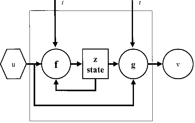
The temporal dynamics of the system, i.e. the transition from state to state, comes about as the state variables are updated by a transition function. The transition function is a causal-determinate function for a determinate system: If the state of a dynamical system at a certain time is known, the state for any other point in time can be computed. Accordingly, the same transition function can be applied for every interval. Its effect is reversible as the effect of time can always be undone by the application of the time evolution function. In this exo-physical concept of time-invariance (Kampis 1994), time is scalar, invariant, reversible and universal. The underlying notion of time is parameter time (Drieschner 1996), derived from absolute Newtonian time, which has the following characteristics (Mittelstaedt 1980, p. 15): Both its topological structure (temporal sequence) and its metric structure (parameter time) are equal. Time has no relationship to objects external to it, while any process refers to the same absolute, universal time (external time).
At the outset of dynamical system building, the set for the encoding of the system is needed. The material object under study is not the system, because every material object contains an unlimited number of variables and, therefore, of possible systems. The system is a list of variables (Ashby 1976, p. 40). The task of the modeler is to vary the list of variables until the system becomes determinate: a determinate machine is one whose behavior can be encompassed in a list of variables that is logically and mathematically workable (Lilienfeld 1978, p. 37). The basic question is which variables are necessary in order to express a given domain of phenomena (Kampis 1992a). Modeling is thus faced with a frame problem (Paton 1996); i.e. the question how reading frames or frames of description should look like (Kampis 1992a).
Notwithstanding the frame problem, an essentialist notion underlies
the dynamical system paradigm: It is assumed that the modeler can discern
the essential properties of the represented system. Modelers pretend to
isolate "
the essential (behaviorally relevant) system structure, i.e.
the identification of essential state variables, their feedbacks, and critical
parameters" (Bossel 1992, p. 264). In this view, the dynamical system retains
the essence of the represented system, i.e. that which remains the
nature of the system throughout its change from potentiality to actuality.
Abstract state and system structure stand for this essence.
Biogeochemical models, the focus of this paper, deal with a range of spatiotemporal scales. At one extreme, inputs and outputs of total landscape units (catchments, watersheds) are measured and modeled. At the other extreme, processes such as decomposition or the nitrogen cycle are studied at the point scale. Models for (agro-)ecosystem management and environmental risk assessment deal e.g. with the dynamics of organic matter (Powlson 1996), the loss of (excess) nutrients such as nitrogen (e.g. de Willigen 1991, de Willigen & Neetson 1985, Engel 1993, Frissel & van Veen 1981, Groot et al. 1991, van Veen 1994) and phosphorous (e.g. Cassell et al. 1998), and with the dynamics of organic contaminants such as pesticides (e.g. Calvet 1995, Richter et al. 1996, Walker 1995) and other xenobiotics (Behrendt 1999).
| Model | Pool |
|
|
|
| SWATNIT | Litter |
|
|
|
| Manure |
|
|
|
|
| Humus |
|
|
|
|
| DAISY | Biomass Pool 1 |
|
|
|
| Biomass Pool 2 |
|
|
|
|
| Soil Organic Pool 1 |
|
|
|
|
| Soil Organic Pool 2 |
|
|
|
|
| AMINO | Humus |
|
|
|
| Fraction 2 |
|
|
|
|
| Fraction 3 |
|
|
|
|
| Fraction 4 |
|
|
|
|
| Fraction 5 |
|
|
|
|
| Fraction 6 |
|
|
|
|
| Fraction 7 |
|
|
|
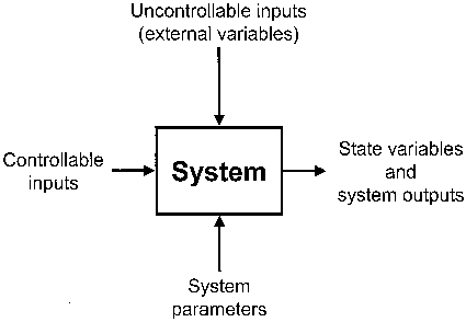
Ecosystem boundaries are usually chosen in such a way that physical factors, e.g. weather and climate, become external variables of the system. The external driving variables are assumed to be independent of the respective ecosystem, i.e. there is no feedback. They presumably propel the ecosystem which, encoded as a dynamical system, reacts to the external variables in a determinate way.
Future weather and climate conditions can not be known a priori, therefore in practice, weather records from the past are used to compute short-term behavior (Addiscott 1993). However, past weather records may be unrepresentative of the full range of natural driving forces (Konikow & Bredehoeft 1992). Particularly when driving forces themselves are subject to major changes (e.g. global climate change) the information content of weather records is invalidated.
3.6 Calibration
Calibration is the attempt to find the best accordance between computed
and observed data by the variation of some selected parameters (Joergensen
1992, p. 68). However, due to the non-identifiability of parameters and
to overparameterization, calibration is a fitting exercise. Therefore,
it is an open question whether it assures predictive capacity and whether
it contributes to understanding (see below).
The validity of the respective set determines the validity of the prediction of system behavior. The encoding of the system in a determined frame of description as in the case of dynamical systems cannot account for the complexity of temporal production of variables (Kampis 1994), which successively invalidates the set. The time frame is crucial here: While in the short run (as indicated by system times, see below) a given set may predict system behavior with a certain degree of accuracy, in the long run self-modifying systems become unpredictable. The encoded abstract system state is outdated by the production of internal novelty. As component systems are self-referential, an external point of reference is lost. The system becomes an endo-system to which an external observer has no access. On large scales, the exo-models thus break down.
The notion of time in self-organizing systems is fairly different from time in dynamical systems. External parameter time is replaced by the concept of endo-time or system time. System time is linked to the period of time a system takes before reproducing (Kümmerer 1996). Hierarchy theory assumes that natural systems can be described in the framework of a nested, constitutive hierarchy (Ahl & Allen 1996, ONeill et al. 1986, Müller 1992). The different levels of organization correspond to different temporal scale levels and to different system times. Accordingly, system times vary from minutes/days (e.g. chemical reactions in soil; molecular level) to months/years (e.g. population dynamics; nutrient cycles) and decades/centuries (e.g. ecosystems, landscapes, global system) (Ulrich 1993). Symmetry breaking in self-organizing systems (Prigogine et al. 1969) entails irreversibility and the notion of structurally determined systems that depend upon their history.
The paradigm of self-modifying systems is non-classical, as these systems are:
| Essentialism
(Reversibility) |
Self-modification
(Irreversibility) |
|
| Being-Becoming | Properties
States |
Relations
Confluences (potentiality) |
| Objects | Objects locally and a priori definable | Objects globally and a posteriori definable (Objects context- and time dependent) |
| Causality | Transparent
Strong Linear |
Opaque
Weak Non-linear; circular |
| System | Dynamical systems
Analytically defined Given hierarchy Closed |
Growing systems
Realistically defined Self-created hierarchy Open |
| Complexity | Constant | Variable |
| Environment | Environment structures system
External regulation (external drivers) |
Systems structure environment
Internal regulation |
| Time | Scalar, universal parameter time (exo-time) | System time (endo-time) |
| Dynamics/
Development |
Reversible trajectories
Continuity Regularity |
Irreversible Process
Bifurcation Singularity |
| Computability | Computable | Non-computable
(Set not definable in advance) |
Theoretical ecologists take different positions with regard to the base model concept. While valid real-structure models are supposed to be achievable in principle (Bossel 1992, Nielsen 1992) others doubt that such representations can be achieved even for simple real ecosystems (Wissel 1989, pp. 1-7); Joergensen (1992) acknowledges that such a base model can never be fully known, because of the complexity of the system and the impossibility to observe all states. In this view, complexity is ontologically conceived and the impossibility of condensing the essence of an ecosystem into a dynamical system is attributed to practical observational and computational (and not principal) limitations.
In the paradigm of self-modification, properties must be envisioned in a relational way as they depend on a changing material context. The notion of a system state has to be abandoned, as states require variables as expressions of the properties of the system. The identity and the definition of the systems components is context and time-dependent and "is only revealed at the end of a process, when all confluences and relations are already known in retrospect" (Kampis 1994).
Modern natural science is based on an exo-physical conception, in which
the material system under study is regarded as a sender and the observer
as a receiver, collecting the signals emitted by the object. This exo-physical
concept collides with the endo-physical notion of self-modifying systems,
which pick up and create information on-line and for which limited internal
accessibility of information is an ontologically conceived factor (Kampis
1994). In such systems, definitions become temporally changeable due to
self-modification; thus, the classical concept of computability where everything
has to be defined in advance ceases to work.
The theory of dynamical systems and its application in empirical sciences, like ecology and the environmental sciences, strives to fit the conception of modern natural science as laboratory science (Hoyningen-Huene 1989). In the laboratory, closed systems are constructed in which if-conditions or antecedents are prepared to produce observable effects or consequences. The corresponding notion of causality is interventionist (Janich 1992) in that intervention in a specific, controlled setting makes causal relationships appear. According to Vicos verum factum principle, truth and understanding are attributed only to systems prepared or created by humans (Hösle 1990). Following Hacking (1992), parts of our environment have to be remade laboriously into a quasi-laboratory to reproduce laboratory phenomena. The dynamical systems approach makes use of process descriptions and of parameters established under laboratory conditions, it aims at the exclusion of noise and tries to achieve a high degree of closure. Thus, the theory of dynamical systems attempts to work with the laboratory model and has indeed been applied successfully to allopoietic, technical systems.
Dynamical systems are the paradigm in the environmental sciences, both as a conceptual background and as the formal base of simulation modeling (Joergensen 1992, Richter 1994, Richter et al. 1996) although the transferability of system analysis and the paradigm of dynamical systems to ecosystems has been questioned in general already two decades ago (Müller 1979). For the following reasons, we consider the dynamical system paradigm inadequate for the representation of ecosystems.
Dynamical systems omit the openness constitutive of ecosystems. Closed dynamical systems run counter to the heterogeneity of ecosystems and to the practical and theoretical limitations imposed on the observation of ecosystems. We agree with the work of Oreskes et al. (1994) who show that ecosystem openness and the formal closeness of dynamical systems collide in three respects: First, dynamical systems require input parameters that are incompletely known (e.g. the distributed parameters). Secondly, they are based on continuum theory that entails a loss of information on structure and processes on finer scales (Oreskes, in press); e.g., the Darcian velocity used for the differential equations is different from the actual velocity at the pore scale. Continuum is a hypothetical idealization, disregarding the discreteness of ecological entities (Breckling 1992). Thirdly, Oreskes et al (1994) show that they recur to additional inferences and assumptions (e.g. kinetic effects are usually neglected), making use of auxiliary hypotheses until the dynamical system and the corresponding simulation model fit the data. Several system structures may produce the same results; i.e. model results are underdetermined by the data.
A dynamical system is an abstraction in which the system is separated from its environment or background. The background is regarded as noise that is eliminated in the abstraction step as only well-defined inputs (the input vector) reach the system. Thus, the system and its input and output vector become a conceptually closed system. The notion of noise is based on a noise/non-noise difference in conjunction with the system/environment difference introduced by information theory and system analysis. Yet in ecology, there are no grounds on which noise (background) and system (abstraction from the background) could be distinguished. Ecosystems and order in ecosystems may actually be the result of noise thus, "noise is music to the ecologist" (Valsangiacomo 1998, p. 270). In system analysis what started out as an ecological system becomes a mere system losing its ecological trait: For ecological issues are issues in which an system-environment-context is structured due to the development of selective behavior of the system towards its environment. The ecological view of a system-environment-context implies unity (of the system-environment difference) despite difference (of system and environment) or even unity due to difference (Luhmann 1990, pp. 21f.).
The differences introduced to abstract a certain system from its context prevent re-unification and unity of context and environment. For example, reintegration of the population-community difference by the process-function difference is impossible. Correspondingly, ecosystem theory has not come up with a single example of successful reconstruction or prediction of both aspects of a given system (Lange 1998).
In dynamical systems, a fixed number of variables are contained. However, the assumption of a fixed number of degrees of freedom collides with the constant come and go of organisms and the generic innovation and extinction in ecosystems along time, resulting in the production of internal novelty, the change of system structure, and the creation and extinction of new variables. In our view, ecosystems have to be regarded as self-modifying component systems, for which the a priori definition of variables is impossible. Internal novelty and constant drift of ecosystems and their components is not noise, but it is essential for the structural coupling of an open system to its environment (Maturana & Varela 1987) and for the structuring of the system-environment context, both in the past and the future. Separation of system and context can at best give a static, momentary view of a frozen system state. Dynamical system modeling of future states assumes that the abstract state and the external parameter time account for a determinate temporal transition. However, self-modifying systems do not transit from one state with determined properties to another determinate state, but are in an incessant process of original self-organization, in which relations are continually established and lost and states are superseded by confluences. No dynamical system can account for this internal novelty and the peculiar system times of system components. For short time frames, dynamical system descriptions may retain validity. In the long run, however, the dynamical system as a reading frame becomes outdated (Kampis 1994).
The notion of reversibility underlying the dynamical system paradigm
implies that any moment in time is equal and that past states can be computed
from present states. The history of the system is supposed to be contained
in the system structure and specific parameters. Such systems are trivial
machines that are synthetically determined, analytically determinable,
predictable, and independent of history, i.e. there is an operator
relating input to output (Foerster 1998). However, the failure of simulation
models is attributed precisely to the ignorance of the historical character
of systems and of system memory (Lange 1998). It has been hypothesized
that sequences in complex systems show non-trivial long-range correlations,
entailing a considerable memory effect (Ebeling et al. 1995, pp.
48-50). Historicity denotes the dependence of the present state of
a system upon its history. The notion of historicity corresponds to the
notion of non-trivial machines, in which the historical record of operations
influences present operations. Non-trivial machines are unpredictable and
in most cases not analytically determinable (Foerster 1998). On top of
that, self-modifying systems are not even synthetically determined. Temporal
dynamics of self-modifying systems are characterized by symmetry breaking,
irreversibility, non-linearity, bifurcations, and evolution. From (the
discovery of) complexity a path is leading to history (Longo 1994).
However, the conventional notion fails for practical and principal reasons. Generally accepted standards for testing and validating ecosystem models are nonexistent. In contrast, current practice is characterized by vague, subjective claims that model predictions show acceptable agreement with data (Kirchner et al. 1996). Validation procedures commonly consist in comparing modeled and measured data or the outputs of different models for the same set of input data. Biogeochemical models for agroecosystems have been validated this way, showing considerable deviation when different model outputs are compared to each other and to measured data (e.g. de Willigen 1991, de Willigen & Neetson 1985, Diekkrüger 1992). Aside from these practical limitations, there are more fundamental shortcomings of the validation procedures in the earth sciences that are discussed by Rastetter (1996). The basal impossibility of the verification and validation of (closed) models of (open) natural systems has been demonstrated by Oreskes et al. (1994).
Measured data used for model calibration and validation do not cover the range of potential conditions of system and external variables, particularly as data usually belong to short-term data sets. Accordingly, model validity is restricted to the range of conditions represented by the respective data set. When this range is surpassed, the predictive capacity of the model is in doubt and can only be confirmed a posteriori; i.e. there is no prediction.
The calibration step, in which models with a large number of non-identifiable
parameters (overparameterization) are fitted to measured data, assures
that models can be adapted to a given data set, irrespective of the internal
structure of the model. Not only are models underdetermined by data (Oreskes
et
al. 1994), they can even become immune to data (Hauhs et al.
1996): eventual lack of predictive power is attributed to the intrinsic
complexity of the system under study, leading at best to a readjustment
of the model (e.g. by the re-calibration of parameters or the addition
of further processes). The role of simulation models as predictive tools
in the environmental sciences and as instruments of decision support has
been harshly criticized for the lack of validity and validation. Mac Lane
(1988) speaks of the construction of massive imaginary future scenarios
to provide predictions that cannot be verified by checking against objective
facts. To him models are speculation without empirical check. Funtowicz
and Ravetz (1992) criticize the absence of effective tests for demonstrating
what sort of correspondence, if any, there is between models and reality.
To them models are devoid of certainty, quality, and reality and are to
be regarded as a post-modern phenomenon. In the absence of testing, models
may take on an aura of reality in the minds of their users (Philip
1991) a particular precarious point if models are employed as risk assessment
tools.
The implications for ecological risk assessment are profound. Unpredictability of natural systems notwithstanding, there are still calls to improve the predictability of biogeochemical system behavior as part of a strategy to reduce global risks, e.g. to decrease the risk of nitrate leaching to the groundwater (WBGU 1999, p. 323). Nevertheless, there is growing awareness that true predictability cannot be achieved. For example, Richter (1994) states that, after repeated application, a faster decomposition of a newly produced pesticide may be explained by the adaptive evolution of the microorganisms, but it can not be predicted. The intrinsic unpredictability of ecosystems suggests following the precautionary principle in risk assessment (Westra 1997), instead of succumbing to the ecosystem engineering fallacy.
However, if dynamical simulation models are not suited for predictive purposes, what role is left to them in the environmental sciences?
We agree with Nancy Cartwrights statement that models are "a work of fiction" and that "some properties ascribed to objects in the model will be genuine properties of the object modeled, but others will be merely properties of convenience" (Cartwright 1983, p. 153). In terms of general modeling theory, the model consists of a set of attributes representing a part of the original and a set of abundant attributes without correspondence to attributes of the original (Stachowiak 1983, p. 119).
Despite not being a real thing, "a model may resonate with nature" (Oreskes et al. 1994) and thus has heuristic value, particular to guide further study. Corresponding to the heuristic function, Joergensen (1995) claims that models can be employed to reveal ecosystem properties and to examine different ecological theories. Models can be asked scientific questions about properties. According to Joergensen (1994), examples for ecosystem properties found by the use of models as synthesizing tools are the significance of indirect effects, the existence of a hierarchy, and the soft character of ecosystems. However, we agree with Oreskes et al. (1994) who regard models as "most useful when they are used to challenge existing formulations rather than to validate or verify them". Models, as sets of hypotheses, may reveal deficiencies in hypotheses and the way biogeochemical systems are observed. Moreover, models frequently identify lacunae in observations and places where data are missing (Yaalon 1994).
As an instrument of synthesis (Rastetter 1996), models are invaluable. They are a good way to summarize an individual research project (Yaalon 1994) and they are capable of holding together multidisciplinary knowledge and perspectives on complex systems (Patten 1994).
While models as a product may have heuristic value, we would like to emphasize also the role of the modeling process: "[ ] one of the most valuable benefits of modeling is the process itself. These benefits accrue only to participants and seem unrelated to the character of the model produced" (Patten 1994). Model building is a subjective procedure, in which every step requires judgment and decisions, making model development half science, half art and a matter of experience (Hoffmann 1997, Hornung 1996). Thus modeling is a learning process in which modelers are forced to make explicit their notions about the modeled system and in which they learn how the analytically isolated components of a system can be glued (Paton 1997). As modeling mostly takes place in groups, modeling and the synthesis of knowledge has to be envisaged as a dynamic communication process, in which criteria of relevance, the meaning of terms, the underlying concepts and theories, and so forth are negotiated. Model making may thus become a catalyst of interdisciplinary communication.
In the assessment of environmental risks, however, an exclusively scientific
modeling process is not sufficient, as technical-scientific approaches
to post-normal risks are unsatisfactory (Rosa 1998) and as the predictive
capacity and operational validity of models (e.g. for scenario computation)
is in doubt. The post-normal science approach (Funtowicz & Ravetz 1991,
1992, 1993) takes account of the stakes and values involved in environmental
decision making. Following a post-normal agenda, model development and
model validation for risk assessment should become a trans-scientific (communication)
task, in which "extended peer communities" participate and in which non-equivalent
descriptions of complex systems are made explicit, negotiated, and synthesized.
In current modeling practice, however, models are highly opaque and can
rarely be penetrated even by other scientists (Oreskes, personal communication).
As objects of communication, models still are closed systems and black
boxes.
In biogeochemical systems, the interplay of biological components with their geochemical environment play a crucial role in the processing of chemical substances. As to this interaction, the paradigm of dynamical systems represents only a halfway discovery of complexity. In our view, the closed encoding of ecosystems as dynamical systems runs counter to the self-modifying character of ecosystems as a result of their singular history in a singular context. As nonstationary systems (self-modification) in a nonstationary context (history), complex natural systems are unpredictable.
While in the environmental sciences a representationalistic notion of
dynamical system models as the product of scientific endeavor prevails,
we emphasize the importance of the modeling process. Modeling can be a
way of coping with different types of complexity: the complexity of integrating
and synthesizing (reductionist) statements and of gluing analytically isolated
components; the descriptive complexity that allows for numerous, non-equivalent
system descriptions, depending upon standpoint; the communicative complexity,
both inter- and trans-scientific, arising from nonequivalent descriptions
of complex systems. Modeling can be a means of reduction of complexity
as it is realizing one arrangement (or agreement) amongst innumerous
contingent arrangements.
Ahl, V.; Allen, T.F.H.: 1996, Hierarchy theory, Columbia Univ. Press, New York.
Arrowsmith, D.K.; Place, C.M.: 1994, An introduction to dynamical systems, Cambridge University Press, Cambridge.
Ashby, W.R.: 1976, An introduction to cybernetics, Chapman & Hall, London.
Behrendt, H.: 1999, Deterministische Modellierung des Stofftransports von organischen Xenobiotika im System Boden-Pflanze, Shaker, Aachen.
Berg, E.; Kuhlmann, F.: 1993, Systemanalyse und Simulation für Agrarwissenschaftler und Biologen, Ulmer, Stuttgart.
Beven, K.: 1996, The limits of splitting: Hydrology, The Science of the Total Environment, 183, 89-97.
Bork, H.-R.; Rohdenburg, H.: 1987, Modellanwendungen zur Analyse der Wasserdynamik landwirtschaftlich genutzter Einzugsgebiete, Verhandlungen des deutschen Geographentages, 45, 439-445.
Bossel, H.: 1992, Real-structure process description as the basis of understanding ecosystems and their development, Ecological Modelling, 63, 261-276.
Bossel, H.: 1997, Allgemeine Systemtheorie und Kybernetik: Systemtheorie dynamischer Systeme, in: Müller, F. (ed.), Handbuch der Ökosystemforschung, EcoMed Verlag, Landsberg.
Breckling, B.: 1992, Uniqueness of ecosystems versus generalizability and predictability in ecology, Ecological Modelling, 63, 13-27.
Calvet, R.: 1995, Modeling pesticide leaching in soils; main aspects and main difficulties, European Journal of Agronomy, 4, 473-484.
Cartwright, N.: 1983, How the Laws of Physics Lie, Oxford Univ. Press, New York.
Cassell, E.A.; Dorioz, J.M.; Kort, R.L.; Hoffmann, J.P.; Meals, D.W.; Kirschtel, D.; Braun, D.C.: 1998, Modeling phosphorus dynamics in ecosystems: Mass balance and dynamic simulation approaches, Journal of Environmental Quality, 27, 293-298.
Casti, J.L.: 1986, On system complexity: identification, measurement, management, in: Casti, J.L. (ed.), Complexity, language, and life, Springer, Berlin & Heidelberg.
De Boer, D.H.: 1992, Hierarchies and spatial scale in process geomorphology. A review, Geomorphology, 4, 303-318.
de Willigen, P.: 1991, Nitrogen turnover in the soil-crop system; comparison of fourteen simulation models, Fertilizer Research, 27, 141-149.
de Willigen, P.; Neetson, J.J.: 1985, Comparison of six simulation models for the nitrogen cycle in the soil, Fertilizer Research, 8, 157-171.
Diekkrüger, B.: 1992, Standort- und Gebietsmodelle zur Simulation der Wasserbewegung in Agrarökosystemen, Vol. 19, Institut für Geographie und Geoökologie der TU Braunschweig, Braunschweig.
Drieschner, M.: 1996, Natur und Wirklichkeit in der modernen Physik, in: Schäfer, L. (ed.), Naturauffassungen in Philosophie, Wissenschaft, Technik, Band IV, Alber, Freiburg, pp. 65-122.
Dubois, D.M. (ed.): 1981, Progress in ecological engineering and management by mathematical modelling: Proceedings of the Second International Conference on the State-of-the-Artin Ecological Modelling sponsored by the International Society for Ecological Modelling (ISEM) and held in Liège, Belgium from 18th to 24th April 1980, Ed. Cebedoc, Liège.
Ebeling, W.; Freund, J.; Schweitzer, F.: 1995, Entropie Information Komplexität. SFB 230, Stuttgart.
Eigen, M.; Schuster, P.: 1979, The hypercycle: a principle of natural self-organization, Springer, Berlin & Heidelberg.
Emmeche, C.: 1994, The computational notion of life, Theoria Segunda Epoca, 9, 1-30.
Emmeche, C.: 1997, Aspects of Complexity in Life and Science, Philosophica, 59, 41-68.
Engel, T.: 1993, Simulationsmodelle zur Stickstoffdynamik, Ulmer, Stuttgart. p. 484.
Foerster, H.: 1998, Entdecken oder Erfinden, in: Gumin, H.; Meier, H. (eds.), Einführung in den Konstruktivismus, Piper, München, pp. 41-88.
Frissel, M.J.; van Veen, J.A.: 1981, Simulation of nitrogen behaviour of soil-plant systems, Center for Agricultural Publication and Documentation, Wageningen.
Funtowicz, S.; Ravetz, J.: 1991, A new scientific methodology for global environmental issues, in: Costanza, R. (ed.), Ecological economics, Columbia University Press, New York, pp. 137-53.
Funtowicz, S.; Ravetz, J.: 1992, The good, the true and the post-normal, Futures, 24, 963-976.
Funtowicz, S.; Ravetz, J.: 1993, Science for the post-normal age, Futures, 25, 739-755.
Gnauck, A.: 1995, Systemtheorie, Ökosystemvergleiche und Umweltinformatik, in: Gnauck, A.; Frischmuth, A.; Kraft, A. (eds.), Ökosysteme, E. Blottner Verlag, Taunusstein, pp. 11-30.
Groot, J.J.R.; de Willigen, P.; Verberne, E.L.J.: 1991, Nitrogen turnover in the soil-crop system, Kluwer, Dordrecht.
Hacking, I.: 1992, The self-vindication of the laboratory sciences, in: Pickering, A. (ed.), Science as practice and culture, University of Chicago Press, Chicago, pp. 29-64.
Haken, H.: 1990, Synergetik: eine Einführung, Springer, Berlin & Heidelberg.
Haken, H.: 1993, The machine as metaphor and tool, Springer, Berlin & Heidelberg.
Hauhs, M.: 1992, Modelle in der Ökosystemforschung, in: DFG (ed.), Regionalisierung in der Hydrologie, VCH, Weinheim, pp. 55-62.
Hauhs, M.; Lange, H.: 1996, Ökologie und Komplexität, Forum für interdisziplinäre Forschung, 16, 46-64.
Hauhs, M.; Lange, H.; Lischeid, G.; Kastner-Maresch, A.: 1998, Möglichkeiten und Grenzen in der Modellierung naturnaher Ökosysteme, in: Dikau, R.; Heinritz, G.; Wiessner, R. (eds.), Global Change, Fr. Steiner Verlag, Stuttgart, pp. 188-206.
Hauhs, M.; Neal, C.; Hooper, R.; Christophersen, N.: 1996, Summary of a workshop on ecosystem modeling: The end of an era?, The Science of the Total Environment, 183, 1-5.
Hedrich, R.: 1994, Die Entdeckung der Komplexität, H. Deutsch Verlag, Frankfurt a. M.
Hoffmann, H.: 1997, Deterministische Modellierung, in: Müller, F. (ed.), Handbuch der Ökosystemforschung, EcoMed Verlag, Landsberg.
Hoosbeek, M.R.; Bryant, R.B.: 1992, Towards the quantitative modeling of pedogenesis a review, Geoderma, 55, 183-210.
Hornung, U.: 1996, Mathematical aspects of inverse problems, model calibration, and parameter identification, The Science of the Total Environment, 183, 17-23.
Hösle, V.: 1990, Vico und die Idee der Kulturwissenschaft, Introduction to: Giambattista Vico, Prinzipien einer neuen Wissenschaft über die gemeinsame Natur der Völker, Meiner, Hamburg, vol. 1, pp. XXI-CCXCIII.
Hoyningen-Huene, P.: 1989, Naturbegriff Wissensideal Experiment, Zeitschrift für Wissenschaftsforschung, 5, 43-55.
Huwe, B.; van der Ploeg, R.R.: 1992, Modellierung des Stickstoffhaushaltes landwirtschaftlich genutzter Böden, in: Kobus, H. (ed.), Schadstoffe im Grundwasser, VCH, Weinheim, pp. 185-230.
Janich, P., 1992: Grenzen der Naturwissenschaft, Beck, München.
Jarvis, P.G.: 1995, Scaling processes and problems, Plant, Cell and Environment, 18, 1079-1089.
Joergensen, S.E.: 1991, Modeling in environmental chemistry, Elsevier, Amsterdam.
Joergensen, S.E.: 1992, Integration of ecosystem theories, Kluwer, Dordrecht.
Joergensen, S.E.: 1994, Models as instruments for the combination of ecological theory and environmental practice, Ecological Modelling, 75/76, 5-20.
Joergensen, S.E.: 1995, State of the art of ecological modeling in limnology, Ecological Modellling, 78, 101-115.
Kampis, G.: 1992a, Information: Course and Recourse, in: Haefner, K. (ed.), Evolution of information processing systems, Springer, Berlin & Heidelberg, pp. 49-64.
Kampis, G.: 1992b, Process, information theory and the creation of systems, in: Haefner, K. (ed.), Evolution of information processing systems, Springer, Berlin & Heidelberg, pp. 85-102.
Kampis, G.: 1994, Biological evolution as a process viewed internally, in: Atmanspacher, H. (ed.), Inside versus outside, Springer, Berlin & Heidelberg, pp. 85-110.
Kauffman, S.A.: 1993, The origins of order, Oxford Univ. Press, New York.
Kay, J.; Schneider, E.: 1995, Embracing complexity: The challenge of the ecosystem approach, in: Westra, L., Lemons, J. (eds.), Perspectives on ecological integrity, Kluwer, Dordrecht, pp. 49-59.
Kirchner, J.W.; Hooper, R.; Kendall, C.; Neal, C.: 1996, Testing and validating environmental models, The Science of the Total Environment, 183, 33-47.
Konikow, L.F.; Bredehoeft, J.D.; 1992, Ground-water models cannot be validated, Advanced Water Research, 15, 75-83.
Kornwachs, K.; Lucadou, W.v.: 1984, Komplexe Systeme, in: Kornwachs, K. (ed.), Offenheit Zeitlichkeit Komplexität, Campus, Frankfurt a. M., pp. 110-166.
Kratky, K.W.; Wallner, F.: 1990, Grundprinzipien der Selbstorganisation, WBG, Darmstadt.
Kümmerer, K.: 1996, The ecological impact of time, Time & Society, 5, 209-235.
Lange, H.: 1998, Are Ecosystems Dynamical Systems?, International Journal of Computing Anticipatory Systems, 3, 169-86.
Lilienfeld, R.: 1978, The rise of systems theory, Wiley, New York.
Longo, G.O.: 1994, Von der Komplexität zur Geschichte, in: Braitenberg, V.; Hosp, I. (eds.), Evolution, Rowohlt, Hamburg, pp. 235-250.
Luhmann, N.: 1990, Ökologische Kommunikation, Westdeutscher Verl., Opladen.
Mac Lane, S.: 1988, Letters, Science, 242, 1623-1624.
Maturana, H.R.; Varela, F.; 1980, Autopoiesis and cognition, Reidel, Dordrecht.
Maturana, H.R.; Varela, F.J.: 1987, Der Baum der Erkenntnis, Goldmann, München.
Mittelstaedt, P.: 1980, Der Zeitbegriff in der Physik, Bibliographisches Institut, Mannheim & Zürich.
Müller, A.M.K.: 1979, Systemanalyse, Ökologie, Friede, in: Eisenbart, C. (ed.), Humanökologie und Frieden, Klett-Cotta, Stuttgart, pp. 250-318.
Müller, F.: 1992, Hierarchical approaches to ecosystem theory, Ecological Modelling, 63, 215-242.
Müller, F.: 1997, State-of-the-art in ecosystem theory, Ecological Modelling, 100, 135-161.
Nielsen, S.N.: 1992, Strategies for structural-dynamic modeling, Ecological Modelling, 63, 91-101.
ONeill, R.V.; DeAngelis, D.L.; Waides, J.B.; Allen, T.F.H.: 1986, A hierarchical concept of ecosystems, Princeton Univ. Press, Princeton/NY.
ONeill, R.V.; Johnson, A.R.; King, A.W.: 1989, A hierarchical framework for the analysis of scale, Landscape Ecology, 3, 193-205.
Odum, H.T.: 1983, Systems ecology, Wiley, New York.
Oreskes, N.: Why believe a computer? Models, measures, and meaning in the natural world, in: Schneiderman, J.S. (ed.), The earth around us, W.H. Freeman, San Francisco (in press).
Oreskes, N.; Shrader-Frechette, K.; Belitz, K.: 1994, Verification, validation, and confirmation of numerical models in the earth sciences, Science, 263, 641-646.
Paslack, R.: 1991, Urgeschichte der Selbstorganisation, Vieweg, Wiesbaden.
Paton, R.C.: 1993, Understanding Biosystem Organisation II: Towards a Theoretical Framework, International Journal of Science Education, 15, 637-653.
Paton, R.C.: 1996, Metaphors, Models and Bioinformation, BioSystems, 38, 155-162.
Paton, R.C.: 1997, Glue, Verb and Text Metaphors in Biology, Acta Biotheoretica, 45, 1-15.
Patten, B.C.: 1994, Ecological systems engineering: toward integrated management of natural and human complexity in the ecosphere, Ecological Modelling, 75/76, 653-665.
Philip, J.R.: 1991, Soils, natural science, and models, Soil Science, 151, 91-98.
Powlson, D.S.: 1996, Evaluation of soil organic matter models, Springer, Berlin & Heidelberg.
Prigogine, I.; Lefever, R.; Golbeter, A.; Herschkowitz-Kauman, M.: 1969, Symmetry breaking instabilities in biological systems, Nature, 223, 913-916.
Rastetter, E.B.: 1996, Validating models of ecosystem response to global change, BioScience, 46, 190-198.
Richter, J.: 1986, Der Boden als Reaktor, Enke, Stuttgart.
Richter, J.; Benbi, D.K.: 1996, Modeling of nitrogen transformations and translocations, Plant and Soil, 181, 109-121.
Richter, O.: 1994, Simulation des Verhaltens von Ökosystemen, in: Bundesministerium für Ernährung, Landwirtschaft und Forsten (ed.), Dynamik und Regulation von Biozönosen im Agrarökosystem, vol. 7. Landwirtschaftsverlag, Münster-Hiltrup, pp. 151-167.
Richter, O.; Diekkrüger, B.; Nörtersheuser, P.: 1996, Environmental fate modeling of pesticides, VCH, Weinheim.
Risser, P.G.M.; Box, E.O.: 1987, Scale effects in landscape studies, in: Turner, M.G. (ed.), Landscape heterogenity and disturbance, Springer, New York & Berlin, pp. 3-14.
Rosa, E.: 1998, Metatheoretical foundations for post-normal risk, Journal of Risk Research, 1, 15-44.
Rykiel, E.J.: 1996, Testing ecological models: the meaning of validation, Ecological Modelling, 90, 229-244.
Stachowiak, H.: 1983, Erkenntnistufen zum Systematischen Neopragmatismus und zur Allgemeinen Modelltheorie, in: Stachowiak, H. (ed.), Modelle Konstruktionen der Wirklichkeit, Fink, München, pp. 87-146.
Toulmin, S.: 1981, Foresight and understanding, Greenwood, Westport/CT.
Ulrich, B.: 1993, Prozeßhierarchie in Waldökosystemen, Biologie in unserer Zeit, 5, pp. 322-9.
WBGU: 1999, Welt im Wandel: Strategien zur Bewältigung globaler Umweltrisiken, Springer, Berlin.
Valsangiacomo, A.: 1998, Die Natur der Ökologie, Hochschul-Verlag an der ETH, Zürich.
van Veen, J.A.: 1994, Modelle zum Stickstoff im Boden: Betrachtungen zum Stand der Forschung, in: Bundesministerium für Ernährung, Landwirtschaft und Forsten (ed.), Bodennutzung und Bodenfruchtbarkeit, Parey, Hamburg, pp. 158-169.
Vereecken, H. et al.: 1991, Comparison of simulation results of five nitrogen models using different datasets, in: European Communities Commission EUR 13501 (ed.), Soil and groundwater research. Report II, Luxembourg, pp. 321-338.
Walker, A.: 1995, Evaluation and improvement of mathematical models of pesticide mobility in soils and assessment of their potential to predict contamination of water systems, BlackwellWissenschaftlicher Verlag, Berlin & Wien.
Westra, L.: 1997, Post-normal science, the precautionary principle and the ethics of integrity, Foundations of Science, 2, 237-262.
Wiens, J.A.: 1989, Spatial scaling in ecology, Functional Ecology, 3, 385-397.
Wissel, C.: 1989, Theoretische Ökologie, Springer, Berlin & Heidelberg.
Yaalon, D.H.: 1994, On models, modeling, and process understanding, Soil Science Society of America Journal, 58, 1276.
Zeigler, B.P.: 1976, Theory of modeling and simulation, Wiley, New York.